Building data pipeline with Apache Airflow – Part 1

    Introduction

    Working on data pipelines is a very essential part of data engineering. One of the key factors of a well-written pipeline is the ‘Orchestration’, which helps automate most of the schedule and dependencies between tasks thus saving a lot of development time. Apache Airflow is one such orchestration tool that has lot of features and 3rd party integrations which makes it very popular among data engineers to manage workflows.

    In this blog (first post of the series), I will share how to install, configure, run and visualize a simple pipeline. So, let’s get started. I have used Postgres as Airflow DB (other options are mysql & sqlite)

    1. Installing Apache Airflow

    mkdir airflow
    cd airflow
    export AIRFLOW_HOME=/absolute/path/to/airflow/directory
    python -m venv venv
    . venv/bin/activate
    pip install apache-airflow
    # optional -- when using Postgres as Airflow metadata DB
    pip install psycopg2-binary
    

    2. Setting Postgres to hold Airflow metadata (default is sqlite)

    /* Execute below commands in your Postgres server */
    CREATE DATABASE airflow_db;
    CREATE USER <airflow-db-user> WITH PASSWORD <airflow-db-pass>;
    GRANT ALL PRIVILEGES ON DATABASE airflow_db TO airflow_user;
    

    3. Configure Airflow to use Postgres as its metadata database

    # Edit "airflow.cfg" file
    # Replace with your values and update the value of 'sql_alchemy_conn' to 
    postgresql+psycopg2://<airflow-db-user>:<airflow-db-password>@<db-host>/airflow_db
    # Save "airflow.cfg"
    # verify DB connection from Airflow
    airflow db check
    # Initialize the DB
    airflow db init
    

    The “db init” command will ensure that Airflow has access to create required tables (It created 28 tables in my Postgres DB)


    4. Create a user to access Airflow webserver

    airflow users create \
        --username admin \
        --firstname Preetdeep \
        --lastname Kumar \
        --role Admin \
        --email no-reply@techwithcloud.com
    

    5. Start Airflow

    # start webserver
    airflow webserver
    # start scheduler
    airflow scheduler
    

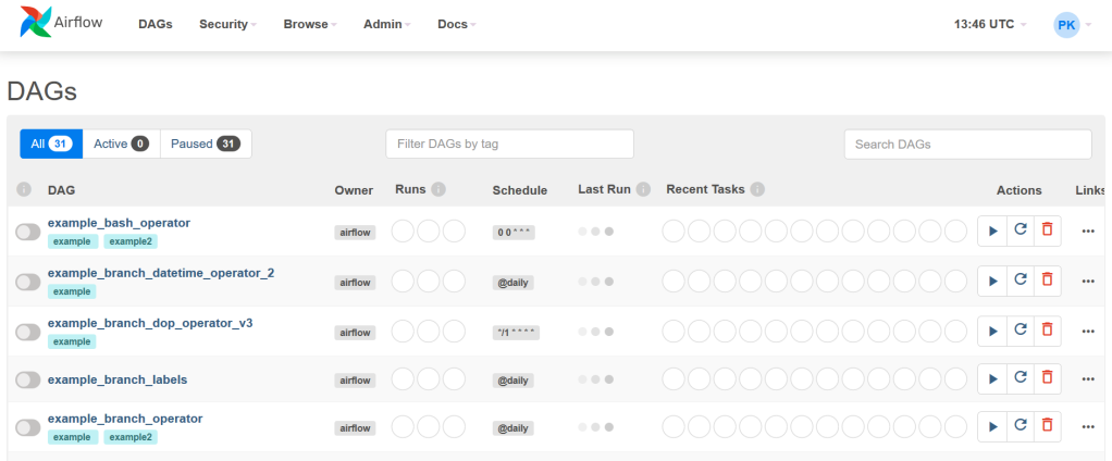
    Now, login to http://localhost:8080 and you should see a page similar to the following. There are some default DAGs defined to play around with. DAG (Directed Acyclic Graph) is a set of tasks (vertices) and their dependencies (edges) in such a way that it doesn’t create a cycle or loop among themselves. In other words, it represents a pipeline (I will use DAG and Pipeline interchangeably).

    Airflow GUI home page with example DAGs

    Now that the basic Airflow setup is complete, time to build a pipeline (DAG). Airflow requires DAGs to be created around “Executors”. The default executor is “SequentialExecutor” which can only run one task instance at a time. For this tutorial, I will be LocalExecutor but for production “CeleryExecutor” is highly recommended.

    There are two types of executor – those that run tasks locally (inside the scheduler process), and those that run their tasks remotely (usually via a pool of workers)

    Airflow Docs

    6. Using LocalExecutor

    Edit "airflow.cfg" file
    Change the value of executor to LocalExecutor
    Save "airflow.cfg"
    # run this command to confirm the change
    airflow config get-value core executor
    

    7. Testing with a demo DAG

    Now that the Airflow environment is configured, let’s execute a simple DAG

    from airflow.operators.python import PythonOperator
    from airflow import DAG
    from datetime import datetime
    
    default_dag_args = {
        'owner': 'techwithcloud',
        'depends_on_past': False,
        'start_date': datetime(2021, 8, 19),
        'schedule_interval':None
        }
    
    # Step 1 = Define tasks
    def task_1():
        print('Hi, I am Task1')
    
    def task_2():
        print('Hi, I am Task2')
    
    # Step 2 = Define a DAG
    with DAG(
        dag_id='simple_dag_demo',
        default_args=default_dag_args,
        tags=['on demand']
        ) as dag:
        
        # Define an operator (encapsulate your tasks)
        t1 = PythonOperator(
                task_id='task_one',
                python_callable=task_1
            )
        
        t2 = PythonOperator(
                task_id='task_two',
                python_callable=task_2
            )
        
        # define lineage
        t1 >> t2
    

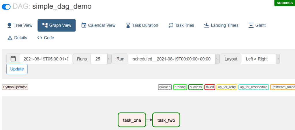
    Save this code as demo_dag.py and copy this file to $AIRFLOW_HOME/dags/ folder. Within few minutes, the Airflow scheduler should detect this new DAG. Refresh your Airflow UI, search for this DAG, activate it and you should see something similar as shown below.

    Airflow: DAG

    To view specific details of a DAG, click on the dag name. I personally find “Graph View” very interesting. From here, you can click on individual tasks and check the logs as well which is very useful in debugging.

    Airflow: Graph view of DAG

    8. Passing data across tasks

    Airflow provides this feature through XCom (short for cross-communication). Marc Lamberti has written a nice blog dedicated to XCom which I highly recommend. The caveat with this approach is that this information should be a small piece of data (key/value pair) under a certain size limit.

    Do not pass sensitive or huge data using XCom

    In the following example (an updated version of the above one), I am using two ways of passing value from one task to another. The first one is using a key and the second one is through the “return” keyword.

    def task_1():    
        ti = get_current_context()['task_instance']
        # push value associated with a key
        ti.xcom_push(key='t1_key', value='t1_xcom_value')
        print('Hi, I am Task1')
        # push value associated with default key
        return 't1_return_value'
    
    def task_2():
        ti = get_current_context()['task_instance']
        # read a value using key and task_id
        xcom_value = ti.xcom_pull(key='t1_key', task_ids=['task_one'])
        # read the returned value of a task
        return_value = ti.xcom_pull(task_ids=['task_one'])
        print('Hi, I am Task2')
        print('Explicit Value {} and Default Value {}'.format(xcom_value, return_value));
    

    Executing this DAG and observing logs for task_2 gives us the following information

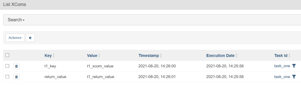
    To view all such XCom key/value pairs from all DAGs, navigate to Admin -> XComs

    Airflow: XComs view

    9. Task Retries and Error Handling

    Airflow provides additional benefits of retrying a task if it has failed during a run. This is super useful when a task has to make HTTP calls or DB connections but should also handle occasional loss of connectivity, busy server, or Throttling.

    # add retry options to default arguments passed to DAG object
    default_dag_args = {
        'owner': 'techwithcloud',
        'depends_on_past': False,
        'start_date': datetime(2021, 8, 20),
        'schedule_interval':timedelta(seconds=15),
        'retries': 3,
        'retry_delay': timedelta(seconds=3),
        'retry_exponential_backoff': True
        }
    
    # raise exception for Airflow to retry
    def task_1():
        ti = get_current_context()['task_instance']
        print('Hi I am task1 from demo dag', ti.try_number)    
        # raise an exception which will trigger retry
        if randint(1, 100) < 50:
            raise AirflowException("Error message")
    

    Executing this new example forces Airflow to retry up to 3 times. You can see the retry attempts in UI by clicking on “Log” in the DAGs details section.

    Airflow: Log by attempts

    Conclusion

    In this post, I shared how to get started with Airflow in a standalone mode. In the next part, I will share how to run a sample ETL pipeline using S3 and Postgres operators.


    References

    1. Setting up a Postgres database for Airflow
    2. DAG Best Practices
    3. Airflow BaseOperator
    4. Airflow PythonOperator

    Monitoring RabbitMQ using Prometheus and Grafana

    Install RabbitMQ

    I followed the instructions provided on the docker hub page here. There are two tags available, I chose the one which had the management plugin pre-configured. This management plugin provides a basic but very helpful management UI for administration. I would recommend having this plugin as default in your RabbitMQ setup but do restrict “HTTP/HTTPS” access to port “15672”. You shouldn’t be exposing RabbitMQ admin console to the outside world.

    docker run -d --name rabbitmq -p 5672:5672 -p 15672:15672 rabbitmq:3.8.16-management
    

    If you are using an older version of RabbitMQ then follow the instructions here to install and configure Prometheus exporter. For this tutorial, I am using the latest 3.8.x version that by default has this plugin.

    As of 3.8.0, RabbitMQ ships with built-in Prometheus & Grafana support.

    https://www.rabbitmq.com/prometheus.html
    # get a prompt to the running container
    docker exec -it rabbitmq /bin/bash
    
    # install curl in the docker container
    apt-get update
    apt-get -y install curl
    
    # verify if rabbitmq_prometheus plugin is installed and enabled -- within container
    curl -v -H "Accept:text/plain" "http://localhost:15692/metrics"
    

    Re run the RabbitMQ container but open access for port 15692

    docker run -d --name rabbitmq \
    -p 5672:5672 -p 15672:15672 -p 15692:15692 \
    rabbitmq:3.8.16-management
    

    Configure Prometheus to scrape RabbitMQ

    Now add this exporter into Prometheus as a target. Edit prometheus.yml file in your Prometheus server directory and add the following entry under scrape_configs. Replace localhost with your RabbitMQ server name.

    scrape_configs:
    - job_name: rabbitmq
      scrape_interval: 60s
      static_configs:
      - targets:
        - localhost:15692
    

    Restart Prometheus service and open Prometheus UI by navigating to http://<hostname&gt;:9090, go to “Status” -> “Targets”, it should show 2 targets now.

    Prometheus UI: Adding RabbitMQ as Target

    Publish and Consume sample messages

    Now that we have RabbitMQ running and configured Prometheus to scrape it, let us create a queue and send some messages before we move to Grafana.

    To create Queue, navigate to RabbitMQ management UI at http://localhost:15672. For this tutorial, I created a queue of type classic using the below settings.

    RabbitMQ: Add a new queue

    Though we can publish and receive messages using management UI, this approach is better suited for queue configuration testing. For this tutorial, I am using the following Python code to publish and consume messages. For full documentation of pika library please see this link.

    Producer for RabbitMQ
    ''' 
    Simple Producer which generates 500 test messages with random delay
    '''
    import pika
    import json
    import random
    from faker import Faker
    from time import sleep
    
    fake = Faker()
    
    connection = pika.BlockingConnection(pika.ConnectionParameters(host='localhost'))
    channel = connection.channel()
    
    # persist messages in case of failure
    msg_prop = pika.BasicProperties(
                delivery_mode = 2, # make message persistent
               )
    
    #send 500 messages with random delay 
    for i in range(1, 500):
        message = {
            "name": fake.name(),      
            "email_id": fake.email(),      
            "address": fake.address()
            }
    
        # Queue was created as durable
        channel.basic_publish(exchange='',
                              routing_key='demo_queue', 
                              properties=msg_prop,
                              body=json.dumps(message))    
        # sleep for few random seconds
        sleep(random.randint(1, 9))
            
    connection.close()
    
    CONSUMER for RabbitMQ
    '''
    Simple consumer to read from the queue with random delay and ack
    '''
    import pika
    import json
    import random
    from time import sleep
    
    connection = pika.BlockingConnection(pika.ConnectionParameters('localhost'))
    channel = connection.channel()
    
    def callback(ch, method, properties, body):    
        print("Received {}".format(json.loads(body.decode())))
        # random delay
        r = random.randint(10, 30)
        sleep(r)
        
        # send ack for only few random messages
        if r%2 == 0: 
            ch.basic_ack(delivery_tag = method.delivery_tag)
    
    channel.basic_consume(queue='demo_queue',                      
                          on_message_callback=callback)
    
    channel.start_consuming()
    connection.close()
    

    Grafana dashboard for RabbitMQ

    You can find detailed information on RabbitMQ client support for various languages here. Now that we have a producer and a consumer (you can run multiple consumers for a single queue), let us configure Grafana which will be our Monitoring and Alerting visualization tool.

    To help Grafana users, RabbitMQ provides few ready-to-use Grafana dashboards (6 as of now). You can create new dashboards and customize existing ones to suit your application’s business need. First, I will import a dashboard called RabbitMQ-Overview into Grafana, which I think is a must-have for any RabbitMQ environment. The steps are given in detail here.

    Grafana: Importing pre-built RabbitMQ Dashboard

    The charts are self-explanatory and very handy when it comes to the visibility of the queues and other components of RabbitMQ. So far, we have configured monitoring for RabbitMQ server and its components, but what about visibility into the underlying VM/Container/EC2 on which this Queue is running.

    Configure cadvisor for Container Metrics

    To have better visibility, we must also monitor at least CPU, Memory and Disk space utilization of the underlying compute infrastructure. For this tutorial I am using docker container to run RabbitMQ so will follow this awesome guide to use cadvisor to monitor container metrics.

    # Pull and run cadvisor container
    docker run \
    --volume=/:/rootfs:ro \
    --volume=/var/run:/var/run:rw \
    --volume=/sys:/sys:ro \
    --volume=/var/lib/docker/:/var/lib/docker:ro \
    --name cadvisor \
    -p 8080:8080 \
    gcr.io/cadvisor/cadvisor
    
    # Update Prometheus config file to scrape the metrics exposed by cadvisor
    scrape_configs:
    - job_name: cadvisor
      static_configs:
      - targets:
        - localhost:8080
    

    Restart Prometheus and navigate to the “Status” section to see that a new target has been added. This tutorial is using localhost for all the setup but you should replace “localhost” with the appropriate IP or Hostname in the prometheus.yml file.

    Prometheus: Scraping container and RabbitMQ metrics

    You can list container metrics with prefix as “container_” and filter based on container name such as shown below. For a full list of cadvisor metrics, please see this doc.

    • container_cpu_usage_seconds_total {name=”rabbitmq”}
    • container_memory_usage_bytes {name=”rabbitmq”}
    • container_memory_max_usage_bytes {name=”rabbitmq”}
    • container_fs_usage_bytes {name=”rabbitmq”}
    • container_fs_limit_bytes {name=”rabbitmq”}

    There are many community-built Grafana dashboards for Prometheus and Docker which you can try or improve upon. I created a sample dashboard to represent 3 metrics for my RabbitMQ container.

    Grafana Dashboard: Container metrics

    Conclusion

    I will strongly recommend configuring alerts in Grafana. Some of the important metrics I will suggest being alerted if they cross a certain threshold are as follows

    1. Unacknowledged Messages
    2. Messages in Queue
    3. Messages Delivered
    4. Connections open
    5. Publishers count
    6. Consumers count
    7. Disk space utilization
    8. CPU utilization
    9. Memory utilization
    Thanks for reading

    Visualize Amazon S3 data using Apache Superset

    Exploratory Data Analysis (EDA) is an important process for many use cases when you are dealing with data. It is much helpful if you get an open-source data exploration and visualization tool that supports a variety of data sources, considering, in the Big Data ecosystem, you always have more than one database. On these lines, I found Apache Superset to be quite impressive and very helpful.

    In this article, I am sharing how to use Superset to explore and visualize data stored in Amazon S3, which is a popular choice for data lake. It took me few iterations to get it to work so hopefully, this post will help people get started.

    Installing Superset

    To install Superset, I followed instructions as mentioned in the docker hub page of superset. However, when I tried to open it in the browser, I got a lot of “Access Denied” errors. After checking these steps and playing with them, I found that “Step 4: Setup roles”, should be done right after “Step 2”. When you load examples before role setting then Superset throws these errors. I have created an issue https://github.com/apache/superset/issues/13867 with the Superset community to fix it.

    So the correct sequence is as follows

    # download docker image and run superset on port 8080
    docker run -d -p 8080:8088 --name superset apache/superset
    
    # With above container running, execute below commands on new terminal
    docker exec -it superset superset fab create-admin \
                   --username admin \
                   --firstname Superset \
                   --lastname Admin \
                   --email admin@superset.com \
                   --password admin
    
    docker exec -it superset superset db upgrade
    docker exec -it superset superset init
    # optional but helpful to get started
    docker exec -it superset superset load_examples
    # save the changes to the image
    docker commit <superset-container-id> apache/superset
    

    Adding Athena Driver in Superset

    Tip – You must have created Athena tables referencing the data in S3. Superset will query Athena tables and use the output for visualization. Since Superset doesn’t access S3 directly, it is transparent to the file format of data stored in S3 (CSV, ORC, Parquet etc).

    As of now, the easiest way to visualize data in S3 is to use Superset’s Athena driver. The complete list of supported DB drivers is published here. For Athena, I am using PyAthena and not the JDBC one. The minimum Dockerfile to pull and build superset image that will include PyAthena connector is shown below.

    FROM apache/superset
    
    # Switching to root to install the required packages
    USER root
    
    # Installing Athena driver
    RUN pip install "PyAthena>1.2.0"
    
    # Switching back to using the `superset` user
    USER superset
    

    Build and run the container again using this updated image. The data used in this article is of a ‘Top 50 Bestselling Books’ on Amazon from Kaggle. As a prerequisite for this tutorial, I created a table in Athena as shown below which points to my S3 bucket having this sample dataset.

    CREATE EXTERNAL TABLE bestseller_books(
      name string,
      author string,
      rating double,
      reviews int,
      price double,
      year int,
      genre string)
    ROW FORMAT SERDE 'org.apache.hadoop.hive.serde2.OpenCSVSerde'
    WITH SERDEPROPERTIES (
      'separatorChar' = ',',
      'quoteChar'     = '"'
    )
    LOCATION 's3://techwithcloud/rawdata/input/'
    TBLPROPERTIES ('skip.header.line.count'='1')
    

    Adding Athena as Database

    Now, login to the Superset UI by opening http://localhost:8080 (default credential is admin/admin) and go to “Data” -> “Databases”. Then click on “+ DATABASE” button, to bring up below page

    Add a DB connection in Superset

    Provide a DB name and the SQLAlchemy URI (connection string) in the following format. Please note that below URI doesn’t contain Athena schema name. Superset will fetch all schema and allows you to choose while creating a dataset. You can find more options to use in the connection string here.

    awsathena+rest://<your_aws_access_key_id>:<your_aws_secret_access_key>@athena.<aws_region>.amazonaws.com/?s3_staging_dir=<path_to_athena_query_output>
    

    As a next step, I recommend going to “SQL Lab” -> “SQL Editor” and selecting the Athena table from the drop down. Superset will automatically fetch few rows (100 rows in my case). If you can see data in the preview then Superset and Athena (or S3) can communicate properly.

    Superset: Preview of Athena Table

    Let us try running a query directly in Superset to find out those authors who had the most number of books sold.

    Superset shows the time taken to execute this query as well as an “Explore” option. Clicking on Explore and following instructions shown on the page brings us to the following very useful section of Superset. Note that till now, we haven’t created any dataset from the table.

    Superset: Exploring SQL query output

    Create Dataset

    Now let us create a dataset from this table. Creating new dataset is very easy, navigate to “Data” -> “Datasets” -> “+ DATASET”. Then select the Athena table, add the dataset. You should see something like below

    Superset: new dataset

    Create Charts

    Now that we have a dataset, let us create 2 charts and add these charts in a dashboard to conclude this tutorial. Navigate to “Charts” -> “+ CHART”, select the dataset name created in the above step, leave the visualization type as “Table”. This brings us to this page where count(*) is the default metric.

    Edit the settings as shown below to get all rows in a table format and save it. This will be our first and simple chart.

    Superset: Table chart having all rows

    For the second chart, I want to see how the books were brought by Genre. Create a new chart and select “Bar Chart” as visualization type. Edit the settings as shown below to create our second chart. Also, in the “CUSTOMIZE” tab, select two check boxes called “SORT BARS” & “LEGEND” and provide labels for the ‘X’ and ‘Y’ axis.

    Adding charts to Dashboard

    So far, we have created 2 charts, and now time to add them to a dashboard.

    1. Navigate to “Dashboards” -> “+ DASHBOARD”
    2. From the “COMPONENTS” tab drag and drop “Row” twice.
    3. From the “CHARTS” tab select the two charts created and drop them in the two Empty Row spaces.
    4. Save the dashboard and you should have a similar page as shown below. (click on the “Draft” icon next to the dashboard name to Publish it to the home page)
    Superset: Dashboard

    This concludes the tutorial. Thanks for reading.

    References

    Building a Simple and Scalable ETL Pipeline for Log Analysis in AWS

    In this article, I share an ETL pipeline that is simple to implement, scalable and provides near real-time analysis of application logs. The data set used is available here https://github.com/logpai/loghub. I have downloaded the Spark log files for this article.

    Overview

    If the log format is well known (e.g. Apache WebServer, Syslog) and in JSON then sending directly to Cloudwatch log group and adding an Elasticsearch publisher is a quick and handy solution. But if the logs are in custom format then it requires correct parsing and conversion to JSON first before ingesting to Elasticsearch. There are two common ways to achieve this.

    a. Agent side – Every compute instances (current or new) running the application code must be also bundled with the conversion logic that will allow an agent reading log lines to know how to parse and convert to JSON before sending it to next stage. This strategy is beneficial when there are manageable number of agents extracting logs and you don’t expect modifications in conversion logic. A drawback is that each agent must be running same version of all types of conversion logic and it should be aware of the type of log lines to apply the correct transformation logic.

    b. Server side – When you receive log lines (in raw format) from multiple agents to a centralized server, then before writing to storage, the conversion logic is applied. Benefit of this approach is to have one location where conversion logic resides and can be updated easily without redeploying or updating remote agents. This is easier to maintain and removes tight coupling between transformation logic and extraction logic. This is the approach I am sharing in this article.

    This article is based on this AWS whitepaper, with focus on use case for

    • Near real-time analysis
    • Ingestion of custom log format
    • Derive custom metric

    The components used in this solution are managed by AWS and thus scale on-demand with no single point of failure.

    ETL pipeline for log monitoring and visualization

    Lambda function for transformation

    First, create a Lambda function that will receive Spark log records (up to max buffer size) from Kinesis Data Firehose. This function will be invoked by the Kinesis and the response will be sent to the destination. Invoking Lambda on in-flight records serves multiple purposes such as transformation, compression, and filtering operation on bulk data in near real-time (min 60 seconds interval).

    The transformation logic I am using is based on an existing lambda blueprint named “kinesis-firehose-process-record-python”. I have modified it to parse a custom log record and convert the output to JSON. The transformation code used in this article is available on Github.

    Tip – Lambda function has a payload limit of 6 MB for both request and response. Ensure Kinesis Data Firehose buffering size for sending request to the function is less than or equal to 6 MB. Also ensure that the response that your function returns doesn’t exceed 6 MB.

    https://docs.aws.amazon.com/lambda/latest/dg/gettingstarted-limits.html

    Create Kinesis Data Firehose delivery stream

    Once we have the lambda function in place the next step is to actually create the Firehose stream. I have used the “–cli-input-json” option to supply input params in a JSON file. These files are available on Github. Please replace it with values from your account before using it.

    # create kinesis data firehose stream using inputs passed in json file (destination as S3)
    aws firehose create-delivery-stream --cli-input-json file://input-to-create-dest-s3.json
    
    AWS console for Kinesis FirehoseDestination as S3

    I recommend to first set S3 as destination and test the data ingestion and transformation using a cool feature in AWS console “Test with demo data”. Other quick option is to use “aws firehose” cli and execute put-record command.

    AWS Kinesis Console – Demo data for testing

    After sending few test data, click on the Monitoring tab to verify if any errors were reported. The transformed record should have been uploaded to destination S3 bucket.

    AWS S3 Console – Transformed Demo data from Kinesis Firehose

    After testing the lambda transformation with test data, delete this delivery stream and the associated test data from S3.

    Deleting Kinesis Firehose delivery stream will not delete the associated destination S3 bucket. It needs to be deleted manually.

    Configuring Elasticsearch cluster

    Now that we have tested our Lambda transformation and Kinesis Firehose using S3, let us create an Elasticsearch cluster to store actual logs data. As a best practice, we will only have logs for a certain time period in elastic (index rotation) and send the raw data into S3 for long-term storage and audit purposes. I strongly recommend creating a bucket lifecycle policy and move older logs to Glacier and/or delete them.

    # create a Cloudwatch log group for publishing logs of new elasticsearch cluster
    aws logs create-log-group --log-group-name /aws/elasticsearch/es-twc
    
    # allow elasticsearch service to create log streams
    aws logs put-resource-policy --cli-input-json file://input-to-es-log-policy.json
    
    # create a Elasticsearch cluster
    aws es create-elasticsearch-domain --cli-input-json file://input-to-create-es.json
    
    # create kinesis data firehose stream using inputs passed in json file (destination as Elasticsearch with backup to S3)
    aws firehose create-delivery-stream --cli-input-json file://input-to-create-dest-es.json
    
    AWS console for Kinesis FirehoseDestination as Elasticsearch

    The Elasticsearch cluster I created is a simple one for tutorial purposes only. It allows connection only from your IP Address. Do not use these settings for production or any such critical / proprietary environment.

    Verifying the ETL pipeline

    So till now, we have verified our Firehose to Elasticsearch pipeline using test data. Now, we will configure the pipeline with log data being sent by Kinesis Agent. The raw logs will go to the S3 bucket and the transformed logs will go to the Elasticsearch cluster with index rotation set to 1 month. To send the sample Spark logs, I have used this simple python function that reads the log file and executes put-record per line.

    After sending some log records, launch Kibana and follow below steps

    1. Navigate to Kibana URL
    2. Go to “Stack Management”
    3. Click “Index Patterns” followed by “Create Index Pattern”
    4. Type the index name in the search bar (in this example it will be staginglogs-*)
    5. Kibana will show the correct index
    6. Click the index and follow the next steps as shown in Kibana UI to complete this process

    After creating index, click “Discover” from main menu and you should see something like following.

    Tips
    1. If the lambda function has an error, then Kinesis will not show any “incoming records” metrics in Cloudwatch. You must check the Lambda function Cloudwatch log groups for errors.
    2. The payload from Kinesis is of type byte after base64 decoding and not String. For any string operation, it must be converted to a string with encoding type (e.g. ‘utf-8’).
    3. When using the transformation function with Kinesis, it is good practice to enable S3 as a backup store for raw log records. This helps in troubleshooting and replaying logs.
    4. Create an Elasticsearch cluster with an index rotation period. This will allow you to quickly search and analyze logs that are hot and most relevant (e.g. Last 2 months), and also managing Elasticsearch cluster cost.
    5. For production and other important environments, always create Elasticsearch cluster in a private VPC without any external access.

    Improving Lambda function to compute custom metric

    Using a transformation function has an additional benefit if you want to filter a bunch of log lines and only interested in specific occurrences of certain keywords. When Kinesis Firehose sends data to Lambda, the response from Lambda is the data that goes to Elasticsearch. This approach is similar to a Window-based computation where Kinesis firehose buffers data (min 1 minute) allowing users to perform custom processing on bulk records. I have shared one such example on Github.

    Cleanup

    Remember to delete the following services used in this tutorial from your AWS console.

    1. Elasticsearch cluster
    2. Kinesis Firehose Delivery Stream
    3. Lambda Function
    4. S3 Bucket or Objects
    5. Cloudwatch Log Groups

    References

    How to transform CSV to Parquet using AWS Glue

    It is no surprise that data storage format play a key role in modern data engineering. You can reduce query time and storage space by selecting appropriate format. We all are familiar with CSV, XML and JSON formats, however there are few limitations when it comes to their application in big data. They do not give much benefit when it comes to aggregation queries or querying against partitioned data. There is no benefit of parallel processing in storing these files on disk (each such file is processed sequentially).

    In such scenarios, a columnar data format speeds up aggregation queries as well as provides space benefit due to better compression techniques. It will be fair to say that two Apache projects Parquet and ORC have won the race for most popular and widely used columnar data format. Both have great support for Hadoop ecosystem and many cloud providers have added these formats into their services.

    In this article, I will share how to transform CSV data into Parquet using AWS Glue. I prefer Glue due to the fact that it is serverless and uses Spark as a compute engine for transformation on input data. AWS Glue has templates for general purpose transformation out of which I will be referring to the one used to convert CSV to Parquet. I prefer Parquet over ORC due to its support for larger block size (128MB).

    The data set used in this tutorial is of an online retail store and publicly available here. I have uploaded the file to an S3 bucket which serves as input bucket.

    Before, we get into Glue let’s try this transformation locally using Spark and Jupyter notebook. After reading the input file into spark data frame, let us observe few lines.

    Fig-1 Showing 5 rows from sample data

    Spark uses Snappy as a default compression technique for Parquet files.

    https://spark.apache.org/docs/2.4.7/sql-data-sources-parquet.html#configuration
    Fig-2 Showing 5 rows from sample data saved in Parquet format

    Looks very easy but not feasible for big data sets which are stored either in a distributed file system like HDFS or Object Storage like S3. AWS Glue is one such service which we can use to automate such transformations steps.

    (1) Create a Table in the Glue catalogue

    You can either manually create a table representing the raw CSV data or better way if to let the Glue crawler scan the input CSV data and create it for you. I used the crawler to scan and create a table which will be source for this tutorial.

    AWS Glue console screenshot – Source table

    This is an external table (or metadata) which is integrated with AWS Athena, thus you can use Athena to query data from this table (our data is in the S3 bucket and will remain there).

    (2) Create a Glue job to transform CSV to Parquet

    Next, we need to create a Glue job which will read from this source table and S3 bucket, transform the data into Parquet and store the resultant parquet file in an output S3 bucket. AWS has made it very easy for users to apply known transformations by providing templates. I will use one such template and run the job.

    Without duplicating myself, I will point you to this AWS blog which shows, how to use Glue Console to create job which will transform CSV files to Parquet. After successful completion of job, you should see parquet files created in the S3 location you provided.

    AWS S3 console screenshot – Parquet file generated by Glue

    In addition to creating parquet file, Glue also allows creating a target table referencing this transformed data set. So you can start using Athena to query parquet data.

    If you are facing issues in running Glue generated job, please check following

    1. Does the IAM role used by Glue has permissions to read/write to desired S3 buckets
    2. Does the S3 bucket uses encryption for which, access to key was not provided to Glue job.
    3. Does your csv file is utf-8 encoded. (this thread)

    Following are excellent blog posts from AWS sharing various techniques around Glue and Spark. I strongly suggest to go through these.

    Couple of other good blogs for references

    AWS Cost – Know your spending before saving

    AWS is not about paying for what you use, it’s about paying for what you forgot to turn off.

    Tweet by Michael Krakovskiy

    Any individual or organization who is using public cloud services (irrespective of the provider) often struggles to recall what they used which resulted in $xyz in their monthly billing invoice. The above tweet summarizes a general feeling of cloud users, that along with “pay-for-what-you-use”, there is an axiom “pay-for-what-you-forget”.

    There are many tips, best practices floating on the Internet on reducing cost so I would not mention them in detail here (AWS has a dedicated page for this topic). Instead, sharing the ones that I observed and found to be a common source of higher cost.

    If you are starting into AWS or planning to expand your cloud services repertoire then use this as a checklist.

    • S3
      • Files uploaded in buckets having version enabled and no lifecycle policy.
      • Lots of services use S3 to store temporary data or output but don’t clean it up when you delete those services.
      • Manual backups of database which is not required anymore but still lying in S3.
    • Athena – Running queries on large CSV data set when you could have used Parquet.
    • Kinesis
      • Too many shards created
      • Not using aggregation when ingesting data.
    • VPC
      • Elastic IPs are allocated but not released after use.
      • Using a high amount of on-demand EC2s instead of using reserve instances.
      • Not using Spot instances for non-critical, fault tolerant tasks
      • Flow logs enabled for the entire subnet or network (should use an appropriate filter)
    • EMR
      • Running jobs on a badly partitioned data set
      • Using unoptimized Spark code
      • Using long running cluster for scheduled batch jobs
    • Others
      • Teams used a bunch of services for proofs-of-concepts but forgot to delete them post demo.
      • Lack of IaC tools like CloudFormation or Terraform, to spin up AWS infrastructure resulting in forgotten & unused services such as SNS topic, Cloudwatch Logs group, Custom Images in ECR repo
      • Long running clusters or databases that are not used 24/7. Do you have identified the access pattern or is there even a process in org which mandates it?
      • Leaving up to individuals to keep track of services they are using or have used in past, but forgot to delete because well people from other teams requested to use it and now no one knows who owns it.

    My answer and tip to all of these are unless you have a cost monitoring and optimization tool (3rd party or offered by AWS), it is not feasible to know the source of high cost and track your usage consistently over a period of time. Instead of once a quarter action item of analyzing cost and asking leads to work with their respective team to reduce cost, why not have a unified view of cost and usage pattern shared with each team (login using SSO).

    AWS is like a Lego box, you need to assemble pieces to build to your application. It grows with your business and then you can’t afford to investigate each service or use another costly service to analyze it. My recommendation is to decide on a tool that provides a single picture of your entire AWS infrastructure, followed by the ability to drill down to each service, calculating its cost and most important “guidelines to save cost based on analyzing historical data” e.g. S3 Intelligent Tier or Trusted Advisor from AWS.

    There is always a trade-off between you paying a cloud provider to offload operations vs hiring engineers to handle operations so that development teams can focus more on building software. I have also observed a hybrid approach by organizations where they are using AWS primarily as IaaS, paying for core compute, storage and networking services while installing and maintaining platforms and/or software on top by themselves. For specialized services, it is on a per need basis or those which have very high operating cost (e.g. Hadoop, Kubernetes).

    In general, your expenditure on cloud providers doesn’t always have to be frown upon. It must reflect the strategic investment you made to have your business grow faster and scale better. So next time when you see your cloud invoice, consider these trade-offs and your business priorities.

    Beginner’s guide to AWS VPC

    I have observed that developers new to AWS, often struggle to understand cloud networking let alone provision a secure Virtual Private Cloud (VPC). Well, with so many frameworks and APIs at your disposal, programming and software development have abstracted to a level that most application developers might not have spent time in understanding networking infrastructure and its impact on applications.

    In this article, I will explain VPC, Subnet, NAT, IGW, Route Tables, etc. to help app developers, not from a networking background, learn basic functioning of these services. I have also included aws commands to provision a secure VPC.

    The deployment architecture to provision is as shown below.

    Sample deployment diagram of a secure VPC

    Virtual Private Cloud (VPC)

    Think of VPC as a virtual network created by AWS for your account. It is completely isolated from VPCs of other users, which allows only you or any AWS account authorized by you to use or modify it. This is your network in the cloud.

    So, why you need VPC? It is required to provision EC2 instances, DB instances, any service running atop EC2, or any compute instances where applications need some sort of network communications. Given the importance of VPC, AWS creates a default VPC for every user in every region. You also get a default Internet Gateway (IGW) attached to the default VPC. As the name suggests, IGW allows you to access the internet within a VPC. It is bidirectional access (source of connection can be either a system on the internet or any EC2 with public IP in VPC).

    VPC is specific to the Region in which it was created. You provide an IP Address range which is in a CIDR notation to create a VPC. I highly recommend getting familiar with CIDR notations and IP Address ranges. Check AWS recommended IPv4 Address Planner to plan subnet CIDR. AWS uses “172.31.0.0/16” as the default in every region. This CIDR range provides 65,534 IP Addresses (2^16) for hosts.

    AWS reserves the first four and the last IPv4 address in each subnet’s CIDR block. They’re not available for use.

    • Network Address: x.y.z.0
    • Router: x.y.z.1
    • DNS: x.y.z.2
    • Reserved for future: x.y.z.3
    • Broadcast: x.y.255.255

    Subnet

    After you have created a VPC, the next logical step is to partition it into subnets. Similar to a traditional network, a subnet represents a logical part of your network and acts as a group with self-contained security policies. Your resource (EC2) virtually resides inside a subnet and communicate to resources in other subnets using route tables.

    Each subnet is associated with a CIDR taken from the parent VPC. A subnet CIDR lets you determine how many private IP Addresses are available for this subnet.

    # Create a VPC using 10.0.0.0/24 as CIDR
    aws ec2 create-vpc --cidr-block 10.0.0.0/24 --tag-specifications ResourceType=vpc,Tags=[{Key=Name,Value=testvpc}]
    
    # Above command will produce a JSON output out of which note the VpcId
    {
        "Vpc": {
            "CidrBlock": "10.0.0.0/24",
              . . .
            "VpcId": "vpc-04bfd0a2f9bb6114a",
    }
    
    # Next create first subnet for public instances (direct route to Internet Gateway)
    aws ec2 create-subnet --vpc-id vpc-04bfd0a2f9bb6114a --cidr-block 10.0.0.0/25 --availability-zone ap-south-1a --tag-specifications ResourceType=subnet,Tags=[{Key=Name,Value=public-subnet-testvpc}]
    
    # Second subnet for private instances (access to internet via NAT Gateway)
    aws ec2 create-subnet --vpc-id vpc-04bfd0a2f9bb6114a --cidr-block 10.0.0.128/25 --availability-zone ap-south-1b --tag-specifications ResourceType=subnet,Tags=[{Key=Name,Value=private-subnet-testvpc}]
    

    These two subnets look as following in the AWS console. Notice that each Subnet, though the allocated quota is of 128 IP Addresses it shows 123 because of AWS reserving 5 IP Addresses. Also, AWS has created a Route Table and Network ACL for our VPC and associated them with new Subnets.

    Screenshot from AWS console

    Internet Gateway (IGW)

    The Internet Gateway allows internet access between instances in VPC and the internet. IGW provides bi-directional or duplex communication and is a fully managed service (horizontally scaled, redundant, and highly available). AWS creates a default IGW and attaches it to your default VPC. This allows users to start accessing their instances created in default VPC from the internet is without much configuration. Internet Gateway is associated with a VPC and not subnets.

    # create a new Internet Gateway (igw) and note down the ID it returned
    aws ec2 create-internet-gateway 
    
    # attach this IGW to new VPC
    aws ec2 attach-internet-gateway --vpc-id vpc-04bfd0a2f9bb6114a --internet-gateway-id igw-00dade6e6f6b3049c
    
    # finally, to allow traffic update the route table for this VPC
    aws ec2 create-route --route-table-id rtb-0fb72edab8223338d --destination-cidr-block 0.0.0.0/0 --gateway-id igw-00dade6e6f6b3049c
    

    So now our route table has a route to Internet via IGW. This route table is by default associated with both subnets hence allowing them to reach the internet and users from internet to reach these two subnets. Let us create a new route table and associate it with private subnet.

    Every new route table is auto-populated to allow traffic within the CIDR (local route)

    # create a new route table and note down the ID
    aws ec2 create-route-table --vpc-id vpc-04bfd0a2f9bb6114a
    
    # associate this route table to private-subnet created above
    aws ec2 associate-route-table  --subnet-id subnet-06bb27a382953fc62 --route-table-id rtb-046b424b6beba4460
    
    # associate the existing route table to public-subnet
    aws ec2 associate-route-table  --subnet-id subnet-0295f8f0c70f7123f --route-table-id rtb-0fb72edab8223338d
    

    Next, we will create a NAT gateway and update the private subnet so that its traffic doesn’t go directly to IGW.

    Network Address Translation Gateway (NAT Gateway)

    It enables instances in a private subnet to connect to the internet or other AWS services, but prevent the internet from initiating a connection with those instances. It helps in abstracting your backend network (private IP Addresses) from public network and denies any traffic not originating from private subnet. The most common use case is when you need to patch servers or download and install software packages from a valid repository. A precondition for NAT is to have an Elastic IP Address (static, public IPv4 address) from AWS.

    # first get an Elastic IP
    aws ec2 allocate-address --domain vpc
    
    # next, create a NAT Gateway (using the allocation-id from above) and associate with public-subnet
    aws ec2 create-nat-gateway --allocation-id eipalloc-0c2ca1171feb46f6c --subnet-id subnet-0295f8f0c70f7123f
    
    # finally, add a route in private-subnet's route table to use NAT Gateway for all IPs
    aws ec2 create-route  --route-table-id rtb-046b424b6beba4460 --destination-cidr-block 0.0.0.0/0 --nat-gateway-id nat-03cc5aa873b4e5d41
    

    In networking, 0.0.0.0/0 represents all IP Addresses. This entry will allow VPC to route any traffic having destination IP Address not matching within 10.0.0.0/24 to the NAT Gateway.

    AWS Console – Entry in route table for NAT Gateway

    Route Tables

    In simple terms, a route table is a lookup table, which defines where to route network traffic. This traffic can be originated from a subnet (within AWS) or the internet. Wait, doesn’t this sound like a Router? You’d be correct in that observation. Please note AWS has a magic router for a VPC but it’s hidden from users and of course, won’t show or give access to their router (which makes perfect sense for a cloud provider). 

    As a user, we can define the routing, using a “route table” for our VPCs and Subnets. An important point here – AWS does not share the physical or virtual interfaces where packets were received (ingress) and from where packets are sent (egress). When a VPC is created, AWS creates a default route table which has an entry ensuring all local traffic is matched and forwarded appropriately. Any subnet created within a VPC is by default associated with a “main route table.”

    VPC Endpoints (Private access to AWS services)

    To further secure network traffic, AWS allows us to create a VPC endpoints, using which instances skip going to Internet and access services like S3 entirely within AWS realm. All the traffic is within AWS network (secured and encrypted) without the need to expose buckets to public. If you are using containers then recommendation is to have an endpoint between your VPC and ECR.

    # create a vpc endpoint of type gateway and associate with public subnet's route table
    aws ec2 create-vpc-endpoint --vpc-endpoint-type Gateway --vpc-id vpc-04bfd0a2f9bb6114a --service-name com.amazonaws.ap-south-1.s3 --route-table-ids rtb-0fb72edab8223338d
    

    The above command does following

    • Create a VPC Endpoint of type Gateway to access an AWS Service, which in this case is “S3” in region ap-south-1
    • Associate the route-table “rtb-0fb72edab8223338d” to this VPC endpoint
    • Add a route in “rtb-0fb72edab8223338d” route table to access the destination service
    AWS Console – VPC endpoint to S3

    Next, to have secure access to ECR, we need to create “Interface” VPC endpoint.

    # used by Docker Registry APIs.
    aws ec2 create-vpc-endpoint --vpc-endpoint-type Interface --vpc-id vpc-04bfd0a2f9bb6114a --service-name com.amazonaws.ap-south-1.ecr.dkr --subnet-id subnet-06bb27a382953fc62
    
    # used by Amazon ECR API
    aws ec2 create-vpc-endpoint --vpc-endpoint-type Interface --vpc-id vpc-04bfd0a2f9bb6114a --service-name com.amazonaws.ap-south-1.ecr.api --subnet-id subnet-06bb27a382953fc62
    
    # to send log information to CloudWatch Logs (used by awslogs log driver)
    aws ec2 create-vpc-endpoint --vpc-endpoint-type Interface --vpc-id vpc-04bfd0a2f9bb6114a --service-name com.amazonaws.ap-south-1.logs --subnet-id subnet-06bb27a382953fc62
    
    AWS console – VPC endpoints

    Network Access Control Lists (NACL)

    The name is self-explanatory as a set of rules which govern the allowed and denies traffic into your subnets. This is a security feature that works at the subnet level and can be thought of as a hidden firewall sitting behind the hidden router. Default NACL allows all inbound and outbound IPv4 traffic but any NACL created by users denies all inbound and outbound traffic until you add rules to allow it.

    There are three parts of NACL that are important to developers:

    • Inbound Rules
    • Outbound Rules
    • Subnet associations

    Rules for both inbound and outbound function independently and must be configured as a pair for bi-direction traffic. In simple terms, if you add an inbound rule to allow HTTP traffic but forgot to add an outbound rule for the same, then AWS will allow incoming HTTP requests but deny HTTP response, causing your application to experience HTTP time-out exception.


    Rules
    are evaluated starting with the lowest numbered rule. As soon as a rule matches traffic, it’s applied regardless of any higher-numbered rule that may contradict it. This is a first-match policy from the lowest rule number to the highest. A rule number marked as “*” matches all traffic, is of the lowest priority and should DENY.

    One of the most common mistakes I have seen in NACLs is to assume the ports for both ingress and egress traffic will be the same. Often the client application uses an ephemeral port. Servers use standard or documented port numbers. So, if you are hosting a web application and allow port 80 for inbound traffic then for outgoing, you should allow all ports or the traffic will not reach the client. Remember inbound needs a source port and outbound needs a destination port.

    Security Group (SG)

    A security group is a more granular level of security feature provided by AWS. It is associated with network interfaces and not with a subnet. When you create an EC2 instance, AWS creates a network interface (eth0) for the EC2 and the security group is associated with this eth0 and not with subnet or EC2. Tomorrow, if you add this interface to a different EC2 instance then the associated SG rules will apply to the new EC2.

    As an analogy, this is a virtual firewall for your compute instances that reside behind the NACL. Users don’t need to configure and maintain both NACLs and SGs; in fact, you will be working with SG more often than NACL because of the default NACL all-allow policy. As with both inbound and outbound rules, AWS creates a default SG when you create VPC.

    Security Groups are different from NACL in the following ways:

    • All rules are evaluated to decide whether to allow or reject
    • There are no “deny” rules, you simply state protocol:port to be allowed
    • For all allowed incoming traffic, SG automatically allows outgoing (stateful firewall) traffic
    • If there is more than one rule for the same port then AWS considers the most permissive rule. According to the documentation: “… if you have a rule that allows access to TCP port 22 (SSH) from IP address 203.0.113.1 and another rule that allows access to TCP port 22 from everyone, everyone has access to TCP port 22.”
    • As a best practice, except for public subnets, be specific in the rules and follow the principle of least privilege.

    Cleanup

    # delete vpc endpoints
    aws ec2 delete-vpc-endpoints --vpc-endpoint-ids vpce-0b1f710745f5d3b27 vpce-09fd7cffd58b6f303 vpce-09f5c94804d5cb3de vpce-015935ad6ee400f77
    
    # delete NAT Gateway
    aws ec2 delete-nat-gateway --nat-gateway-id nat-03cc5aa873b4e5d41
    
    # release Elastic IP used to create NAT Gateway
    aws ec2 release-address --allocation-id eipalloc-0c2ca1171feb46f6c
    
    # delete VPC created for this tutorial
    aws ec2 delete-vpc --vpc-id vpc-04bfd0a2f9bb6114a
    

    In case, you are facing difficulty from the command-line then login to AWS console and delete the components.

    This article is an updated version of my blog published here.

    References

    How to load partitions in Amazon Athena

    Many teams rely on Athena, as a serverless way for interactive query and analysis of their S3 data. One important step in this approach is to ensure the Athena tables are updated with new partitions being added in S3. This allows you to transparently query data and get up-to-date results.

    In this article, I will share few approaches to load partitions with their pros and cons. This list is not exclusive, you should implement a design that best suits your use case.

    The data set used as an example in this article is from UCI and publicly available here. I uploaded few sample files to an S3 bucket with single partition as “s3://techwithcloud/rawdata/retail/dt=yyyy-mm-dd/file<number>.csv”. To monitor Athena API calls to this bucket, a Cloudtrail was also created along with a Lifecycle policy to purge objects from query output bucket.

    -- Create table in Athena to read sample data which is in csv format.
    CREATE EXTERNAL TABLE IF NOT EXISTS retail_rawdata (
      Invoice INT,
      StockCode STRING,
      Description STRING,
      Quantity INT
    )
    PARTITIONED BY (dt string)
    ROW FORMAT DELIMITED
    FIELDS TERMINATED BY ','
    LOCATION 's3://techwithcloud/rawdata/retail'
    TBLPROPERTIES (
        'skip.header.line.count'='1'
    );
    

    1. MSCK REPAIR TABLE

    After creating a table in Athena, first step is to execute “MSCK REPAIR TABLE” query. This is also the simplest way to load all partitions but quite a time consuming and costly operation as the number of partitions grows. Besides, Athena might get overloaded if you have multiple tables (each mapping to their respective S3 partition) and run this query frequently for each table. Athena will add these queries to a queue and executes them when resources are available. This thread in Athena forum has good discussion on this topic.

    A newly created Athena table will have no records until partitions are loaded.

    Athena shows zero records for SELECT query of a newly created table
    -- Load all partitions
    MSCK REPAIR TABLE retail_rawdata;
    
    Athena shows this message after running MSCK REPAIR TABLE
    -- Running SELECT query again
    select * from retail_rawdata limit 5;
    
    After loading partitions output of SELECT query with limit 5

    Note – The partitioned column is part of SELECT query output even though it was not specifically provided as a column inside the create table statement block.

    Running “MSCK REPAIR TABLE” again without adding new partitions, won’t result in any message in Athena console because it’s already loaded. Next, I checked Cloudtrail logs to verify if Athena did any Get/List calls (since this partition is part of meta store now).

    As per the Cloudtrail logs, every call to “MSCK REPAIR TABLE” results in Athena scanning the S3 path (provided in the LOCATION). It does a ListObjects on S3 path and then for each partition executes a HeadObject followed by ListObjects (irrespective of partition loaded or not). As and when new partitions are added, this will take time and add to your cost thus a naive way of loading partitions.

    2. ALTER TABLE ADD PARTITION

    Another way to add partitions is the “ALTER TABLE ADD PARTITION” statement. In this approach, users need to provide the partition value(s) which they want to load. This eliminates the need to scan all the S3 prefixes but requires users to have some mechanism that tracks new partition values to be loaded.

    -- Load single partition
    alter table retail_rawdata add partition(dt='2020-12-22');
    
    -- Load multiple partitions
    alter table retail_rawdata add 
    partition(dt='2020-12-22')
    partition(dt='2020-12-23');
    

    An intuitive approach might be to pre-compute partition value (if it follows a pattern e.g. date, timestamp) and preemptively run “ALTER TABLE ADD PARTITION” every fixed interval. This hack may not work in real-world use cases because data doesn’t always arrive in order & sorted by partition values. As an example, a partition with value dt=’2020-12-05′ in S3 will not guarantee that all partitions till ‘2020-12-04’ are available in S3 and loaded in Athena. You must anticipate an out of order delivery.

    Note – A partition needs to be loaded in Athena only once, not for every file uploaded under that partition.

    3. ALTER TABLE ADD PARTITION with S3 Event Notification and Lambda

    Loading partitions in Athena using S3 event notification

    Instead of users tracking each partition, a cloud-native approach will be to leverage S3 bucket event notification in conjunction with Lambda. For every “s3:ObjectCreated:Put” (or s3:ObjectCreate:*”) event, filtered for the partitioned object prefix, S3 will call a lambda function passing the full prefix. This lambda will then submit an “Alter Table Add Partition” query to Athena.

    A sample lambda function (using python and boto3 library) to submit this query to Athena.

    import boto3
    import os
    from botocore.config import Config
    from urllib.parse import unquote_plus
    
    db_name = os.environ['DB_NAME']
    table_name = os.environ['TABLE_NAME']
    query_output = os.environ['QUERY_OUTPUT']
    
    config = Config( retries = { 'max_attempts': 2, 'mode': 'standard' } )
    athena = boto3.client('athena', config=config)
    
    def submit_to_athena(partition_name):
        query = 'ALTER TABLE {table} ADD PARTITION ({partition})'.format(table=table_name, partition=partition_name)
        response = athena.start_query_execution(
                        QueryString=query,
                        QueryExecutionContext={
                            'Database': db_name
                        },
                        ResultConfiguration={
                            'OutputLocation': query_output
                        }) 
        return response['QueryExecutionId']
    
    def lambda_handler(event, context):
        # Records is array but it will always have one record 
        # when used with S3 bucket event notification
        record = event['Records'][0]
        key = unquote_plus(record['s3']['object']['key'])
        partition = key.replace('rawdata/retail/', '').split('/')[0].replace('dt=','')
        athena_job_id = submit_to_athena('dt=\''+ partition +'\'')
        print('athena_job_id='+athena_job_id)
    
    # create an event notification for S3 bucket
    aws s3api put-bucket-notification-configuration --bucket techwithcloud --notification-configuration file://notification.json
    
    # content of notification.json
    {
        "LambdaFunctionConfigurations": [
            {
                "Id": "NewPartitionEvent",
                "LambdaFunctionArn": "arn:aws:lambda:ap-south-1:2008XXXXXXXX:function:AthenaLoadPartition",
                "Events": [
                    "s3:ObjectCreated:*"
                ],
                "Filter": { "Key": {  "FilterRules": [ { "Name": "Prefix", "Value": "rawdata/retail" } ] } }
            }
        ]
    }
    

    Added few partitions in S3, the “History” tab of Athena console confirms Lambda function executed successfully.

    Screenshot from Athena History showing queries called from Lambda

    Pros – Fastest way to load specific partitions. Doesn’t require Athena to scan entire S3 bucket for new partitions. Suitable when creation of concurrent partitions is less than the limit on Lambda invocations. Ideal if only one file is uploaded per partition.

    Cons – Since S3 will invoke Lambda for each object create event, it might throttle lambda service and Athena might also throttle. If multiple files are uploaded to single partition then the lambda function needs to either send the same partition value again or add a check to see if partitions are loaded or not.

    4. ALTER TABLE ADD PARTITION with Persistent Store and Lambda

    All the 3 approaches discussed so far, assume that each call to Athena will succeed and thus don’t track if the partitions were successfully loaded or not (must wait for Athena’s response). If any error during loading, then those partitions values should be retry. To achieve this, some sort of persistent storage is required where all the newly added partitions and query execution id from Athena should be saved till they are successfully loaded or max_retry is reached.

    Similarly, if a partition is already loaded in Athena, then ideally it should not be called again. In cases when multiple files are uploaded in the same partition, each object creation will result in an event notification from S3 to Lambda. Though there won’t be an impact on tables because Athena will throw an exception and fail the query.

    There are multiple options to improve the previous design, out of which I will discuss two approaches, one using Queue and another using a DB.

    4.1 Using Queue

    In this approach, a queue can be used to collect events from S3 and another queue to store the query execution id along with partition value. The message will be deleted only when that partition was loaded successfully else it should be put back in the queue for later retry.

    I will use SQS as an example here because of S3 native support for event notification. This design has the benefits of using only 2 lambda functions at any given point of time (scheduled using Cloudwatch). There are few caveats such as; max 10 messages per poll & processing duplicates records, because in many real-world scenarios a partition folder in S3 will have multiple files uploaded.

    Athena Load Partitions – S3, SQS, Lambda
    1. Every ObjectCreate event to rawdata S3 bucket triggers an event notification to SQS Queue-1 as destination.
    2. First Lambda function (scheduled periodically by Cloudwatch), polls Queue-1 and fetches max 10 messages.
    3. Parse message body to get partition value (e.g. dt=yyyy-mm-dd), call “Alter Table Load Partitions” and get the query execution id.
    4. Send the query execution id and the message to SQS Queue-2 and delete this message from Queue-1
    5. Second Lambda function (scheduled periodically by Cloudwatch), polls SQS Queue-2
    6. Lambda-2 checks the query execution status from Athena.
    7. Delete message from SQS Queue-2 if status was Success or Failed.
    8. If query state was “Failed” but reason is not “AlreadyExistsException”, then add the message back to SQS Queue-1

    There are no charges for Data Definition Language (DDL) statements like CREATE/ALTER/DROP TABLE, statements for managing partitions, or failed queries.

    https://aws.amazon.com/athena/pricing/

    Another option can be to add SQS trigger for lambda function. This design will result in a lot of lambda functions being invoked (one per event) and the same key prefix being sent to multiple functions. I prefer to control the invocation of Lambda functions such that at any given point of time only one lambda is polling SQS thus eliminating concurrent receiving of duplicate messages. Having 1 consumer for SQS simplifies a lot of things.

    Sample code for both lambda functions is available on github.

    Note – After configuring SQS as a destination for S3 events, an “s3:TestEvent”, is generated and sent by S3. Be careful to remove this message from the queue or add a logic in Lambda to ignore such messages.

    4.2 Using Database

    In this approach, a DB is used to store the partition value (primary key), query_execution_id, status and creation_time. This solution will add some cost as compared to previous ones but a major benefit of this design is that you don’t need to write additional logic to prevent loading same partition value again. Besides, almost every solution has some sort of database (RDS or self-managed), thus an existing DB instance can be leveraged for this use case.

    Athena Load Partitions – S3, SQS, Lambda, RDS

    An SQS Queue is used to collect records directly from S3 for every “ObjectCreate” event. Another option is to invoke Lambda directly from S3 but additional logic needs to be coded to handle throttling errors & DLQ. Using a Queue in between S3 and Lambda provides benefit of limiting Lambda function invocation as per use case, and also a limited number of concurrent writes to RDS to reduce exhausting DB connections.

    -- Sample table creation in PostgreSQL 
    CREATE TABLE athena_partitions
    (
        p_value character varying NOT NULL,
        query_exec_id character varying,
        status character varying NOT NULL DEFAULT '',
        creation_time timestamp NOT NULL DEFAULT NOW(),
        PRIMARY KEY (p_value)
    );
    

    Our first lambda function (scheduled using Cloudwatch), will poll SQS and get max 10 messages. It will extract the partition values and do a bulk UPSERT operation (INSERT IF NOT EXISTS)

    -- Postgresql
    INSERT INTO athena_partitions (p_value) VALUES ('dt=2020-12-25'), ('dt=2020-12-26')
    ON CONFLICT ON CONSTRAINT athena_partitions_pkey DO NOTHING;
    

    A Second Lambda function (scheduled from Cloudwatch) will perform a select operation

    --Read rows where partition values are not loaded completely
    SELECT p_value FROM athena_partitions WHERE status == '' OR status == 'STARTED' LIMIT 10;
    

    For rows returned, where status == ” the function will call “Alter Table Load Partitions” and update the row with status=’STARTED’ and the query execution id from Athena.

    --Sample update in PostgreSQL after receiving query execution id from Athena
    UPDATE athena_partitions 
    SET
      query_exec_id = 'a1b2c3d4-5678-90ab-cdef', 
      status = 'STARTED' 
    WHERE
      p_value = 'dt=2020-12-25'
    

    For rows returned where status == ‘STARTED’ the function will check query execution status from Athena and update the status accordingly. A failed status means empty status.

    --Sample update in PostgreSQL if loading failed (to be retried later)
    UPDATE athena_partitions 
    SET
      status = '' 
    WHERE
      p_value = 'dt=2020-12-25'
    

    To Delete rows, I recommend to have either a cron job or another Lambda function, that will run periodically and delete rows having “creation_time” column value older than ‘X’ minutes/hours. The value of ‘X’ depends on your use case, i.e. when should you expect all files of a partitions to be available in S3 (e.g. 1 hour, 12 hours, 7 days)

    You can find nice examples to connect & query from RDS in the references below.

    References

    Thanks for reading, welcome your feedback.

    Data Security with AWS Key Management Service – Part II

    In the previous post, I shared the workflow for symmetric key encryption. This article will focus on a workflow for asymmetric keys for encryption, digital signing and verification in AWS Key Management Service (KMS). While a symmetric key is mostly used in the context of Data at Rest where data is owned by a singular entity/team, an asymmetric key is used mostly in the context of Data in Transit where data is transferred between two entities.

    An asymmetric key (using different keys for encryption and decryption) has the following main benefits

    • Separates the process of encryption and decryption between two keys. A private key is never shared with the outside world and thus private to the owner, whereas the public key can be safely shared.
    • A key pair enables establishing trust between entities. Only a correct private key (thus a valid entity) can decrypt a message which was encrypted using its public key.
    • A sender can digitally sign messages (or documents) with their private key. The receiver can verify the integrity of the message using the sender’s public key.

    How to Encrypt using asymmetric CMK in KMS

    The first step is to create an asymmetric Customer Master Key (CMK) in KMS. As of now, AWS restricts usage of this CMK to either encryption/decryption OR sign/verify but not both. However, a generated data key pair can be used for both purposes.

    # Creating Asymmetric CMK for Encryption and Decryption using default option of AWS creating the key material
    aws kms create-key --description "a-cmk for EncryptAndDecrypt" --key-usage ENCRYPT_DECRYPT --customer-master-key-spec RSA_4096 --origin AWS_KMS
    
    # Above command returns following output
    {
        "KeyMetadata": {
            "AWSAccountId": "2008XXXXXXXX",
            "KeyId": "3edcaa6f-6d34-4887-afff-7c5eb35fd772",
            "Arn": "arn:aws:kms:ap-south-1:2008XXXXXXXX:key/3edcaa6f-6d34-4887-afff-7c5eb35fd772",
            "CreationDate": "2020-12-17T23:56:33.398000+05:30",
            "Enabled": true,
            "Description": "ToEncryptAndDecrypt",
            "KeyUsage": "ENCRYPT_DECRYPT",
            "KeyState": "Enabled",
            "Origin": "AWS_KMS",
            "KeyManager": "CUSTOMER",
            "CustomerMasterKeySpec": "RSA_4096",
            "EncryptionAlgorithms": [
                "RSAES_OAEP_SHA_1",
                "RSAES_OAEP_SHA_256"
            ]
        }
    }
    

    The private key of an asymmetric CMK, never leaves AWS KMS unencrypted.

    # Download the public key, decode from base64, save it in file
    aws kms get-public-key --key-id 3edcaa6f-6d34-4887-afff-7c5eb35fd772 --output text --query PublicKey | base64 --decode > public_key.der
    

    Any data submitted to the Encrypt, Decrypt, or Re-Encrypt APIs that require use of asymmetric operations must also be less than 4KB.

    https://aws.amazon.com/kms/faqs/
    # To encrypt, use "encrypt" API and and pass the CMK key id. KMS encrypts using your public key.
    aws kms encrypt --key-id 3edcaa6f-6d34-4887-afff-7c5eb35fd772 --plaintext fileb://data.txt --encryption-algorithm RSAES_OAEP_SHA_256 --output text --query CiphertextBlob | base64 --decode > data.cipher
    
    # To decrypt, use "decrypt" API and pass the same CMK key id. KMS decrypts using your private key.
    aws kms decrypt --key-id 3edcaa6f-6d34-4887-afff-7c5eb35fd772 --ciphertext-blob fileb://data.cipher --encryption-algorithm RSAES_OAEP_SHA_256 --output text --query Plaintext | base64 --decode > recover_data.txt
    

    How to Encrypt using asymmetric data key pair

    If for any reason, you do not want to use asymmetric CMK or want to use the same key pair for encryption and sign/verify then the data key pair is a better option. KMS protects the private data key under symmetric CMK.

    There is a limit on max data size which can be encrypted by RSA (as explained here). To overcome this limit, a hybrid encryption process is used (explained here). Assuming if both parties have access to each other’s public key then-

    • The sender generates a random symmetric key
    • Encrypt large data with this symmetric key
    • Encrypt the random symmetric key using the receiver’s public key
    • Share the encrypted data and encrypted random key to the receiver
    • The sender then removes the random symmetric key from local storage and memory

    Tip – To generate data key pair, KMS only needs symmetric CMK key id (or alias) and key pair type. The symmetric CMK is used by KMS to encrypt and decrypt private data key. KMS does not use a private master key for the encryption of data keys.

    https://docs.aws.amazon.com/kms/latest/developerguide/concepts.html#data-key-pairs
    # Generate Data Key pair without receiving plaintext private key. 
    # This command returns plaintext public key and encrypted private key (as base64 encoded). 
    # Copy and save them in a file (e.g. public_key.base64, private_key_cipher.base64) 
    aws kms generate-data-key-pair-without-plaintext --key-id alias/twc/cmk --key-pair-spec RSA_4096
    
    # Decode and save the public data key (which was returned as plaintext) in a file
    openssl enc -d -base64 -A -in public_key.base64 -out public_key.der
    
    # Then use above output to encrypt the actual data (max 4 KB)
    openssl rsautl -encrypt -in data.txt -inkey public_key.der -keyform DER -pubin -out data.encrypted
    

    Asymmetric encryption workflow

    Asymmetric encryption workflow using KMS data key pair with S3 as storage option

    How to Decrypt using asymmetric data key pair

    # Decode the base64 encrypted private data key and save in a file
    cat private_key_cipher.base64 | base64 --decode > private_key.cipher
    
    # Use above file to get plaintext private data key from KMS. Remember to pass the correct symmetric CMK key id
    aws kms decrypt --key-id alias/twc/cmk --ciphertext-blob fileb://private_key.cipher --output text --query Plaintext > private_key_plaintext.base64
    
    # Decode this base64 plaintext private key and save in a file
    openssl enc -d -base64 -A -in private_key_plaintext.base64 -out private_key.der
    
    # Finally decrypt the data
    openssl rsautl -decrypt -in data.encrypted -inkey private_key.der -keyform DER -out recoverdata.txt


    Asymmetric decryption workflow

    Asymmetric decryption workflow using KMS data key pair with S3 as storage option

    How to sign and verify messages using AWS KMS

    In the context of data-in-transit, a very important use case is to first ensure the message (or document) received is the same as the source (not a single bit was changed) and secondly, the message was sent by the person who claims to be the source. Digital signature and verification solves both of these requirements of message integrity and trusted identity. KMS provides a way for users to perform digital signature and verification of messages either in the AWS realm through CMK itself or outside AWS using generated data key pair.

    # Create an asymmetric CMK to sign and verify. This can't be used for encryption and decryption.
    aws kms create-key --description "SignAndVerify" --key-usage SIGN_VERIFY --customer-master-key-spec RSA_4096
    
    # Above command produces following output
    {
        "KeyMetadata": {
            "AWSAccountId": "2008XXXXXXXX",
            "KeyId": "1f5ea5c2-f216-4dcc-9145-99323ec2cb86",
            "Arn": "arn:aws:kms:ap-south-1:2008XXXXXXXX:key/1f5ea5c2-f216-4dcc-9145-99323ec2cb86",
            "CreationDate": "2020-12-19T17:25:35.168000+05:30",
            "Enabled": true,
            "Description": "ToSignAndVerify",
            "KeyUsage": "SIGN_VERIFY",
            "KeyState": "Enabled",
            "Origin": "AWS_KMS",
            "KeyManager": "CUSTOMER",
            "CustomerMasterKeySpec": "RSA_4096",
            "SigningAlgorithms": [
                "RSASSA_PKCS1_V1_5_SHA_256",
                "RSASSA_PKCS1_V1_5_SHA_384",
                "RSASSA_PKCS1_V1_5_SHA_512",
                "RSASSA_PSS_SHA_256",
                "RSASSA_PSS_SHA_384",
                "RSASSA_PSS_SHA_512"
            ]
        }
    }
    

    KMS provides a single key id or alias which internally references both public and private key

    # To sign any data, we need to use "sign" KMS API, then base64 decode and save it in a file
    aws kms sign --key-id 1f5ea5c2-f216-4dcc-9145-99323ec2cb86 --message fileb://document.txt --signing-algorithm RSASSA_PKCS1_V1_5_SHA_256 --output text --query Signature | base64 --decode > signature
    
    # Now, the sender will encrypt "document.txt" with the receiver's public key.
    # Then send both encrypted message and signature to an AWS user with access to kms:Verify API
    
    # To verify, a receiver will first use their private key to decrypt the document
    # Then call "verify" KMS API on the document and signature files
    aws kms verify --key-id 1f5ea5c2-f216-4dcc-9145-99323ec2cb86 --message fileb://document.txt --signature fileb://signature --signing-algorithm RSASSA_PKCS1_V1_5_SHA_256
    
    #Above command produces the following output
    {
        "KeyId": "arn:aws:kms:ap-south-1:2008XXXXXXXX:key/1f5ea5c2-f216-4dcc-9145-99323ec2cb86",
        "SignatureValid": true,
        "SigningAlgorithm": "RSASSA_PKCS1_V1_5_SHA_256"
    }
    

    Tip – KMS doesn’t require downloading or sharing a public key to verify a message signed by asymmetric CMK itself. It needs a valid key id (or alias) and type of signing-algorithm used by the sender.

    Use cases for using KMS CMK for sign/verify

    • The key access is controlled by IAM and audited by Cloudtrail
    • Can be used with cross-account CMK
    • Following inputs needs to be known to the AWS user verifying the message
      • key-id or key alias
      • signing-algorithm
      • kms:Verify permission on the key
    • Upto 4 KB of message can be signed
    • For data more than 4 KB, AWS recommends the following
      • Sender creates a digest (e.g. SHA256), then creates a signature of the digest.
      • Receiver needs to first create a digest (using the same algorithm) of the data, then verify this hash.
    • My suggestion is to maintain a git repo of cryptography related utility code that is shared among all teams.
    • For large data, a common pattern is to securely uploaded data and signature in a S3 bucket (SSE-S3 enabled), along with key alias and signing-algorithm added in the metadata.

    How to sign and verify messages using OpenSSL (or outside KMS)

    There are situations, where the person verifying the data is not an AWS user or doesn’t have access to KMS API. In such cases, teams can use KMS as a central service to generate data key pairs and share the public key to the receiver. The signing will be done at your end not using KMS API but some other crypto libraries available to both parties. OpenSSL is one such very popular and commonly used library. Similarly, the receiver will use your public key to verify the message using OpenSSL or any such standard library.

    Though KMS doesn’t track data key usage (inside or outside of AWS), it will still log the API call made to generate data key pair.

    # Assuming you have generated and saved the data key pair from KMS as shown in the previous example
    
    # Sender signs the message and creates a file called data.signature
    openssl dgst -sha256 -sign private_key.der -keyform DER -out data.signature data.txt
    
    # Receiver verifies the message with sender's public key
    openssl dgst -sha256 -verify public_key.der -keyform DER -signature data.signature data.txt
    
    # above command produces (if the message integrity is not compromised and the sender is the right entity)
    Verified OK
    
    # if in case the data.txt was compromised or the public key is different/invalid then OpenSSL will show the following output
    Verification Failure
    
    digital sign and verify workflow

    References

    1. https://github.com/awsdocs/aws-kms-developer-guide/blob/master/doc_source/importing-keys-encrypt-key-material.md
    2. https://awscli.amazonaws.com/v2/documentation/api/latest/reference/kms/index.html
    3. https://docs.aws.amazon.com/kms/latest/developerguide/symm-asymm-choose.html#key-spec-rsa
    4. https://docs.aws.amazon.com/kms/latest/developerguide/download-public-key.html
    5. https://docs.aws.amazon.com/kms/latest/developerguide/concepts.html#data-key-pairs
    6. https://www.openssl.org/docs/man1.0.2/man1/openssl-dgst.html

    Thanks for reading, welcome your feedback.

    How to save cost in AWS Athena using CREATE TABLE AS SELECT

    Amazon S3 (Simple Storage Service) is a very common and popular choice when it comes to a cheap, durable and highly available data lake. Quite often, teams want to interactively query big data sets directly from S3 for a variety of use cases. Amazon Athena helps users by providing a serverless option using standard SQL to run ad-hoc queries.

    Athena charges by data scanned per query, which as of writing this post is $5 per TB rounded to 10 MB for us-east. For big data sets that are in CSV for JSON format, cost of Athena queries can go North. Converting into a columnar format to save cost is well documented out of which CTAS is one such option that doesn’t require creating and running Spark jobs in AWS EMR.

    In this article, I share use cases and few limitations when using CTAS, short for CREATE TABLE AS SELECT to convert data set into a columnar format and save cost. The example used in this article is based on a publicly available Covid-19 data set.

    To begin with, let us upload this raw data to an S3 bucket.

    C:\> aws s3 cp covid19-eu.csv s3://techwithcloud/rawdata/ --sse
    upload: .\covid19-eu.csv to s3://techwithcloud/rawdata/covid19-eu.csv

    I also created a CloudTrail to monitor the Read and Write API calls for this bucket to examine Athena calls to S3. Next, create a table in Athena for this raw data set.

    CREATE EXTERNAL TABLE IF NOT EXISTS covid19_rawdata (
      `date` DATE,
      day SMALLINT,
      month SMALLINT,
      year SMALLINT,
      cases INT,
      deaths INT,
      countryname STRING,
      geoId STRING,
      countrycode STRING,
      popData2019 BIGINT,
      continentExp STRING,
      cases_per_100K_for_14d DOUBLE
    )
    ROW FORMAT DELIMITED
    FIELDS TERMINATED BY ','
    LOCATION 's3://techwithcloud/rawdata/'
    TBLPROPERTIES (
        'skip.header.line.count'='1'
    );
    

    Run a query to get new cases per month per continent from this data set.

    SELECT query on CSV data set

    Next, create a new table in Athena using CTAS pattern and configure the output as “Parquet with Snappy compression”. I prefer Parquet because it has a bigger block size as compared to ORC.

    CREATE TABLE IF NOT EXISTS covid19_parquet
      WITH (
        format='PARQUET',
        parquet_compression = 'SNAPPY',
        external_location='s3://techwithcloud/parquetdata'
      ) AS SELECT * FROM covid19_rawdata
    

    Now running the same query on this table produces the following

    SELECT query on Parquet data set

    As you can see the amount of data scanned with parquet is 567 KB as against 4 MB scanned in raw CSV data (saving of about 13%). Since Athena charges for data scanned, this a pretty decent saving. AWS has written a nice blog on Athena performance tuning which will help the case to use a columnar format (e.g. Parquet) for cost-saving.

    Distribution of Athena API calls to S3

    Now, let us examine the Cloudtrail logs to see how many API calls were made to S3 by Athena (after all, these calls are chargeable too).

    I had executed 2 queries, the first was “CREATE TABLE AS SELECT” and the second was a “SELECT”. After loading the Cloudtrail logs in Elasticsearch and visualizing them in Kibana, I saw total of 35 entries when filtered for "userIdentity.invokedBy":"athena.amazonaws.com" with the majority of calls being GetObject followed by HeadObject.

    CTAS use cases

    • Short-term queries on huge data set e.g. Security team wants to audit logs every quarter and require access for 2 weeks.
    • Repeated queries on the same data set for specific time e.g. QA team would like to run multiple queries on last month’s data.
    • Queries involving specific columns from huge data set e.g. Data Science team is interested in only 8 columns and not interested in other 20 columns. Once the model is trained, they don’t require to query this data.

    Limitations

    • Even though compressed, there will be two copies of data (one is source raw data and another is the parquet file created as a result of the CTAS query. As per this AWS blog, a 1 TB Elastic Load Balancer (ELB) logs data resulted in 130 GB compressed Parquet files. This looks good athena saving but if these parquet files are leftover then you will be charged an extra $3 per month in this example. This might become hundreds of dollars for production data.
    • If new data is uploaded in S3, then you have to options
      • Delete your existing parquet file from S3 and rerun the CTAS query
      • Use “INSERT INTO” to add new data in your existing Parquet table
    • Loading new partitions in the source rawdata table doesn’t effect CTAS table
    • Not specific to CTAS but related to Athena in general. It doesn’t delete temp files in S3 on your behalf. You must create a bucket lifecycle policy to avoid being charged for Athena files, you don’t require any more.

    Conclusion

    CTAS pattern is a pretty good choice to convert raw data into a columnar format and save Athena cost that requires much less overhead. However, it is more suitable for use cases involving short term analysis of huge data set and not to be used as CSV/JSON to Parquet conversion step in data pipeline.

    Thanks for reading, welcome your comments/feedback.